#database
# 1. Cost model
- 通过预估来决定哪个 plan 更好(不需要实际运行)。
- 是一种内部统计,数值在不同 DBMS 之间不具有可比性。
- 预估可以通过统计不同资源的消费:
- **CPU**:开销小,很难估算
- **Disk**:多少 block transfers
- **Memory**: DRAM读取量
- **Network**:多少 messages
- 预估读/写了多少 tuples
---------
# 2. Statistics
- 为了实现预估成本,DBMS在内部 catalog 里存储了关于 tables、attributes、indexes 等内部统计信息。
- 不同的系统可能在不同时机更新统计信息,也可以通过手动方式触发。
> 更新一般需要全表扫描,代价很大,对于 OLTP 系统可能选择在请求低峰时进行。
- 对于每个关系 R,DBMS 维护了以下信息:
- $N_R$:R 中有多少 tuples
- $V(A, R)$:R 中关于列 A 有多少 distinct values
## 2.1 Derivable Statistics
- **Selection cardinality**
- 记作 $SC(A,R)$ ,表示列 A 等于某一个值的平均有多少行记录。即 $N_R/V(A,R)$。
- 问题:**data uniformity**
## 2.2 Selection Statistics
- unique keys 的相等条件容易预估:
```SQL
SELECT * FROM people
WHERE id = 123;
```
这是简单的 predicate。
### Complex Predicates
- 一个谓词 **P** 的 selectivity(**sel**) 是值符合条件的元组数量与总数量之比。
- 计算方式取决于谓词的类型:
- 相等(Equality)
- 范围(Range)
- 不等(Negation)
- Conjunction
- Disjunction
- **Equality Predicate**
- 谓词为列A = constant,如 `SELECT * FROM people WHERE age = 2`
- $\large sel(A=constant)\ =\ SC(P)\ / \ N_R$ // 假设分布均匀
- **Range Predicate**
- $\large sel(A >= a) \ = \ (A_{max}-a)\ / \ (A_{max}-A_{min})$
- **Negation Predicate**
- $\large sel(not\ P)\ = \ 1- sel(P)$
> $\large Selectivity\ \approx \ Probability$
- **Conjunction**
- $\large sel(P1 \wedge P2) = sel(P1) \times sel(P2)$
- 假定谓词之间是相互独立的(independent)
- **Disjunction**
- $\begin{aligned} \large &sel(P1 \vee P2) \\ &\ \ = sel(P1) + sel(P2) - sel(P1 \wedge P2) \\& \ \ = sel(P1) + sel(P2) - sel(P1) \times sel(P2) \end{aligned}$
- 同样, 假定谓词之间是相互独立的(independent)
- 前面讨论的假定前提条件:
- **Uniform** **Data**:每个 value 的分布是相同的
- **Independent Predicates**
- **Inclusion Principle**:join keys 的 domain 是重叠的,即 inner relation 的每个 key 在 outer 中也有对应的
### Correlated Attributes
^1b06de
示例:一个关于汽车的 database
- Makes = 10,Models=100
考虑以下查询:
- `(make = "Honda" AND model = "Accord")`
如果假定谓词之间相互独立且分布均匀,则 selectivity 为:
$1/10 \times 1/100 = 0.001$
而实际上只有 Honda 会生产 Accord 型号,所以实际的 selectivity 为:
$1/100 = 0.01$
## 2.3 Cost Estimations
### Histograms
- **背景**:
- 数据往往分布不均匀;
- 为每个 distinct value 维护一个 count 代价非常高;
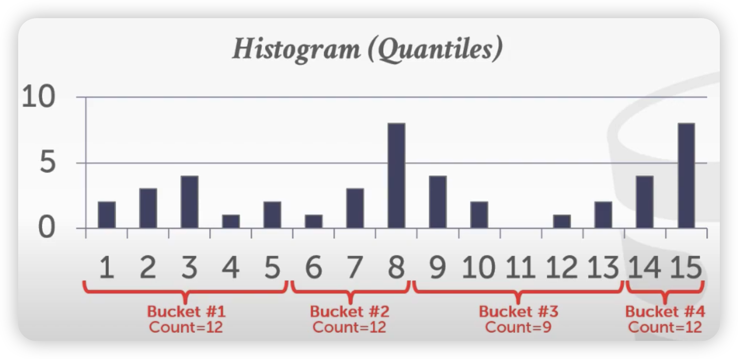
- **Histogram Ranges**
- 每 N 个 values (width)划分为一个 bucket,统计该 bucket 内所有 values 出现的次数(counts)。
- 问题:bucket 内可能有些 values 特别频繁,有些特别不频繁,造成有些 values 统计失真严重
- **Quantiles**
- bucket 的宽度 width 是变化的,让每个 bucket 的 counts 总和是几乎一样的
- 
<br>
### Sampling
- smaller copy of table(如每个100行采样一条数据)
<br>
- 用途:估算 selectivities
<br>
- 对比直方图:
- 直方图更快,Sampling使用时需要 sequential scan
> SQL Server:简单查询使用直方图,复杂查询使用 smapling
-----------
# 3. Query Optimization
- 执行完 RBO后,DBMS 会枚举不同的 plan,然后估算它们的成本:
- **单表**,如 predicate 顺序选择
- **多表**,如 N-way join
- **嵌套子查询**
然后穷举所有 plans 或者到达一定时限后 来挑选最好的
<br>
## 3.1 Single Relation Query Planning
- 挑选最好的 access method:
- 顺序扫描 Sequential Scan
- 二分搜索(clustered indexes)
- Index scan
- Predicate evaluation ordering:谓词应用的顺序选择
### OLTP Query Planning
- 比较简单,一般查询的数据很小,且常常是单点查询。
> sargable( Search Argument Able)
- 通知只需要挑选最好的索引就行
- Join 几乎都是基于外键,且基数很小
- 可以基于一些启发式机制来实现
## 3.2 Multi-Relation Query Planning
- Join 变多,可供选择的 plans 急速变大
> **需要限制 search space**
- Join 基本策略:只考虑 left-deep join trees
- System R 中实现
- 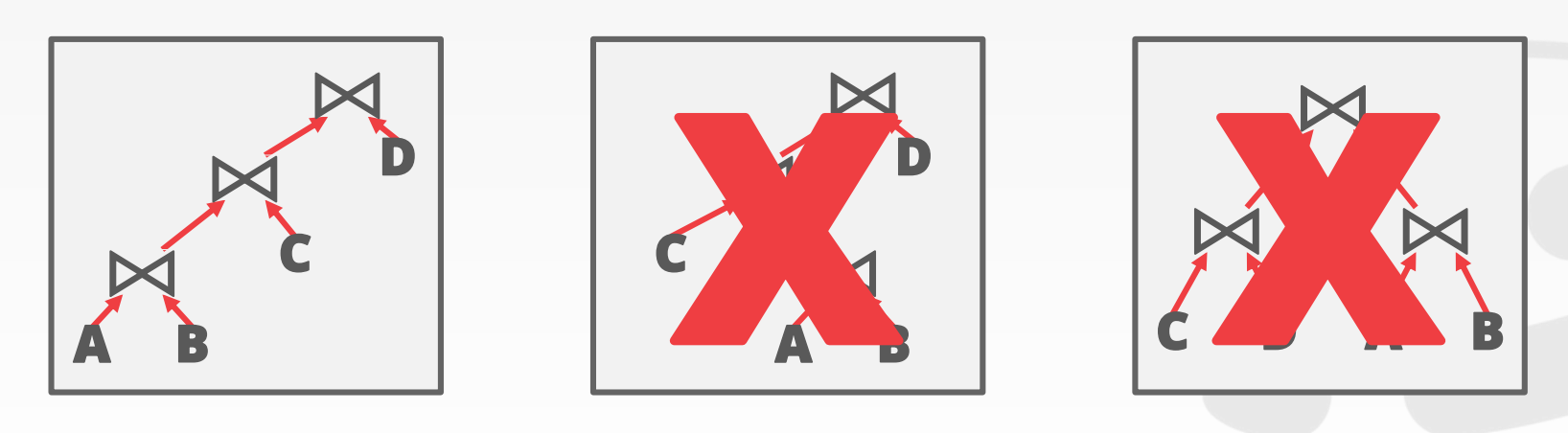
- 优势:允许 fully pipelined plans,中间结果不需要写入临时文件。
> 但不是所有的 left-deep tree 都是 fully pipelined。
- **如何枚举 query plans**:
- 枚举 orderings(逻辑层面)
- 如多表 Join 顺序
- 为每个 operaotr 枚举 plan
- Hash、Sort-Merge、Nested Loop,...
- 枚举每个 table 的 access paths
- Index、Seq Scan
- 使用 **dynamic programming** 来减少 cost estimations 的数量
- 每次挑选 lowest cost for path
## 3.3 Postgres Optimizer
支持两种:
- Dynamic Programming
- Genetic Query Optimizer(GEQO。复杂场景下使用)
> 查询中的 tables 数量小于 12 时使用第一种,大于等于 12 时使用 GEQO。
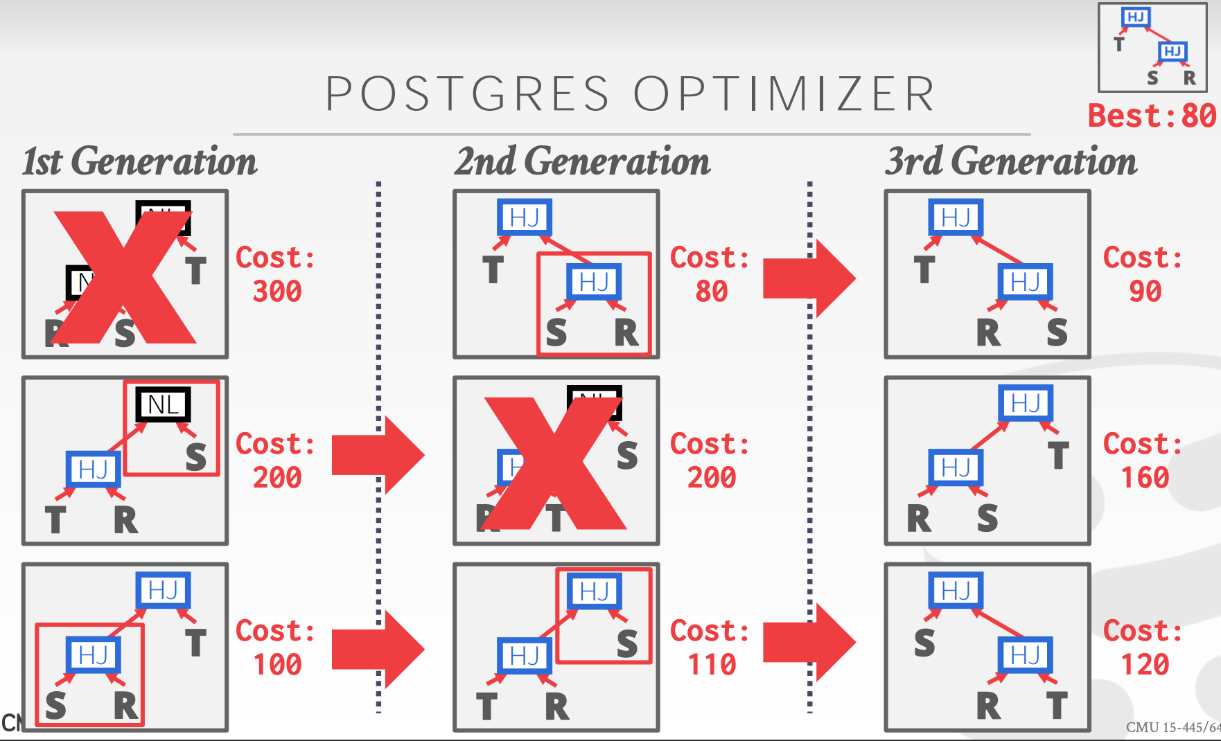
- 靠随机生成第一代
- 每一代剔除最差的,同时记录下最好的(跟全局最好的进行比较更新)
- 剩下的相互混合,生成下一代
--------------
# 4 Nested Sub-Queries(Rewrite)
- DBMS 将 Where 语句中的嵌套子查询看作是一个函数:
- 接受参数
- 返回一个或者一组 values
- 两种方式(rewrite阶段,不需要 CBO):
- Rewrite to de-correlate and/or flatten them
- Decompose nested query and store result to temporary table
- **de-correlate**
```SQL
SELECT name FROM sailors AS S
WHERE EXISTS (
SELECT * FROM reservers AS R
WHERE S.sid = R.sid
AND R.day = '2018-10-15'
)
```
重写为 Join:
```SQL
SELECT name
FROM sailors AS S, reservers AS R
WHERE S.sid = R.sid
AND R.day = '2018-10-15'
```
- **decomposing**
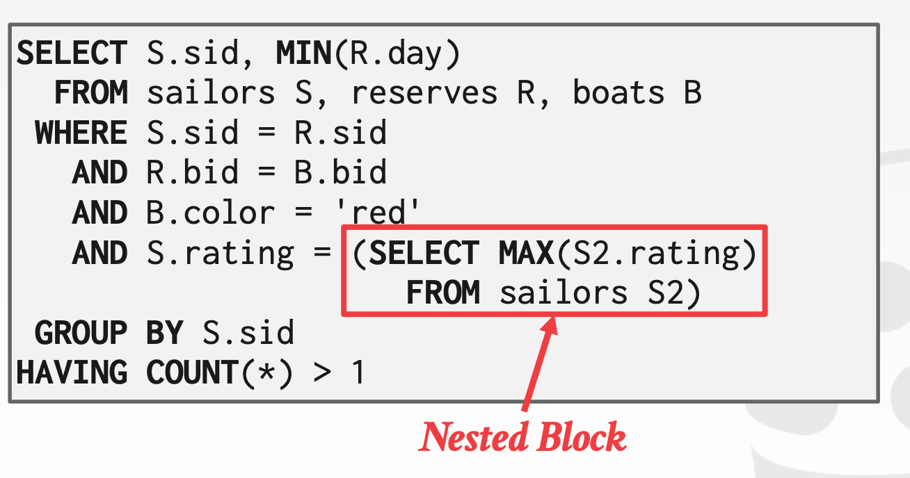
- 将子查询执行,替换为执行结果。
实现方式:optimizer 将查询分割为 blocks,然后连接不同 blocks
- 好处:子查询不用每遍都执行。