- OLAP 不需要像 OLTP 一样索引单个 tuple，文件通常也是不可变的。 - **Sequential Scan Optimizations**： - Data Prefetching / Scan Sharing - Task Parallelization / Multi-threading - Clustering / Sorting - Late Materialization - Materialized Views / Result Caching - Data Skipping - Data Parallelization / Vectorization - Code Specialization / Compilation - **Data Skipping** - **方式一：Approximate Queries（Lossy）** - 在整个表的一个采样子集上进行查询，输出近似结果 - 示例：BlinkDB，[Redshift](https://docs.aws.amazon.com/redshift/latest/dg/r_COUNT.html)，ComputeDB，XDB，[Oracle](https://oracle-base.com/articles/12c/approximate-query-processing-12cr2)，[Snowflake](https://docs.snowflake.com/en/user-guide/querying-approximate-frequent-values)，[BigQuery](https://cloud.google.com/bigquery/docs/reference/standard-sql/approximate_aggregate_functions?hl=zh-cn)，[DataBricks](https://docs.databricks.com/sql/language-manual/functions/approx_count_distinct.html) - **方式二：Data Pruning（Loseless）** - 使用辅助数据结构，根据谓词快速判断可以跳过哪部分数据 - DBMS 需要在 scope 与 filter efficacy、manual 与 automatic 之间进行权衡 - scope vs. filter efficacy：两个极端：为整个 table 建立 min/max 对比 为每个 tuple 建立 - manual vs. automatic：如 zone maps 通常是自动维护的，bitmap 一般需要手动创建 <br> - **Data Considerations** - **Predicate Selectivity**：满足某个查询谓词的有多少 tuples - **Skewness**：某列所有的值都是不同的 或者 包含了许多重复的值 - **Clustering / Sorting**：某个查询条件涉及到的列是否已经排好序 ------------ # 1. Zone Maps - 为一个 block 内的 tuples 预先计算一些聚合信息。DBMS 首先查看 zone map 来判断是否需要访问该 block。 - 最初称为[ Small Materialized Aggregates（SMA）](https://www.vldb.org/conf/1998/p476.pdf) - DBMS 自动地创建/维护 - **Scope vs. filter efficacy trade-off** - 如果 scope 太大，则 zone maps 变得无用 - 如果 scope 太小，则 DBMS 需要花费太多时间来检查 zone maps - Zone Maps are only useful when the target attribute's position and values are correlated. 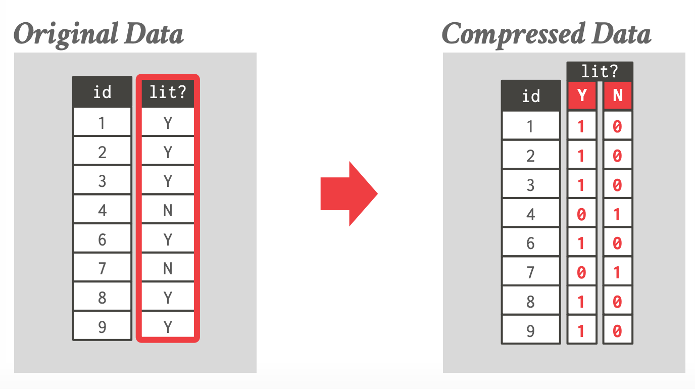- 反例：比如 values 分布完全随机，检查每个 block 的 zone map 时都返回 true ------ # 2. Bitmap Indexes - 为每个不同的列值维护一个 bitmap，bitmap 里存储哪些行包含该列值 - bitmap 的 $i^{th}$ 为 1 表示第 $i^{th}$ tuple 的拥有该列值 - 通常划分为 chunks 来避免分配大块连续的内存。  ## 2.1 Design Choices - **Encoding Schema** - 如果在一个 Bitmap 内表示和组织数据 - 本节课主要涉及 - **Compression** - 如何减少稀疏 Bitmaps 的大小 ## 2.2 Encoding 几种方式： - **Equality Encoding** - 最基本方式，每个不同的值对应一个 Bitmap - **Range Encoding** ^9b6f0f - 每个区间对应一个 Bitmap。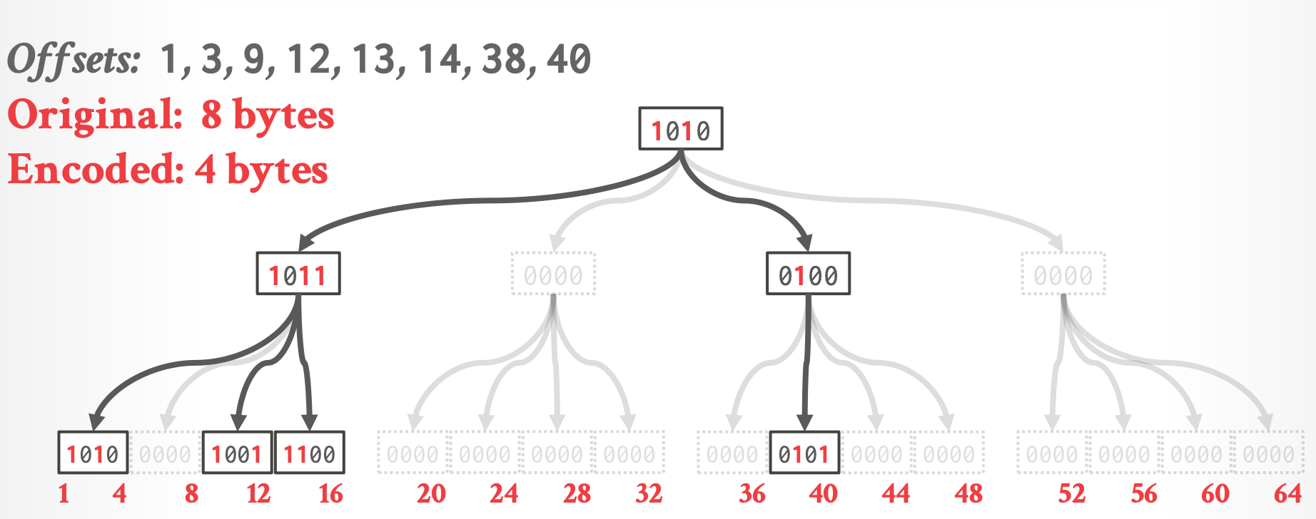**存在 false positive** - 示例：[PostgreSQL BRIN](https://www.postgresql.org/docs/current/brin-intro.html) - **Hierarchical Encoding** - 使用 tree 结构来表示空的 key ranges - **Bit-sliced Encoding** - Use a Bitmap per bit location across all values ## 2.3 Hierarchical Encoding  - 每个 node 自身也是一个 bitmap，第 N 位表示它的第 N 个 child 是否为空 - 虚线的部分不存储 **缺点**： - 对现代 CPU 不友好，访问的内存不连续（许多 indirection） ## 2.4 Bit-Sliced Encoding  - 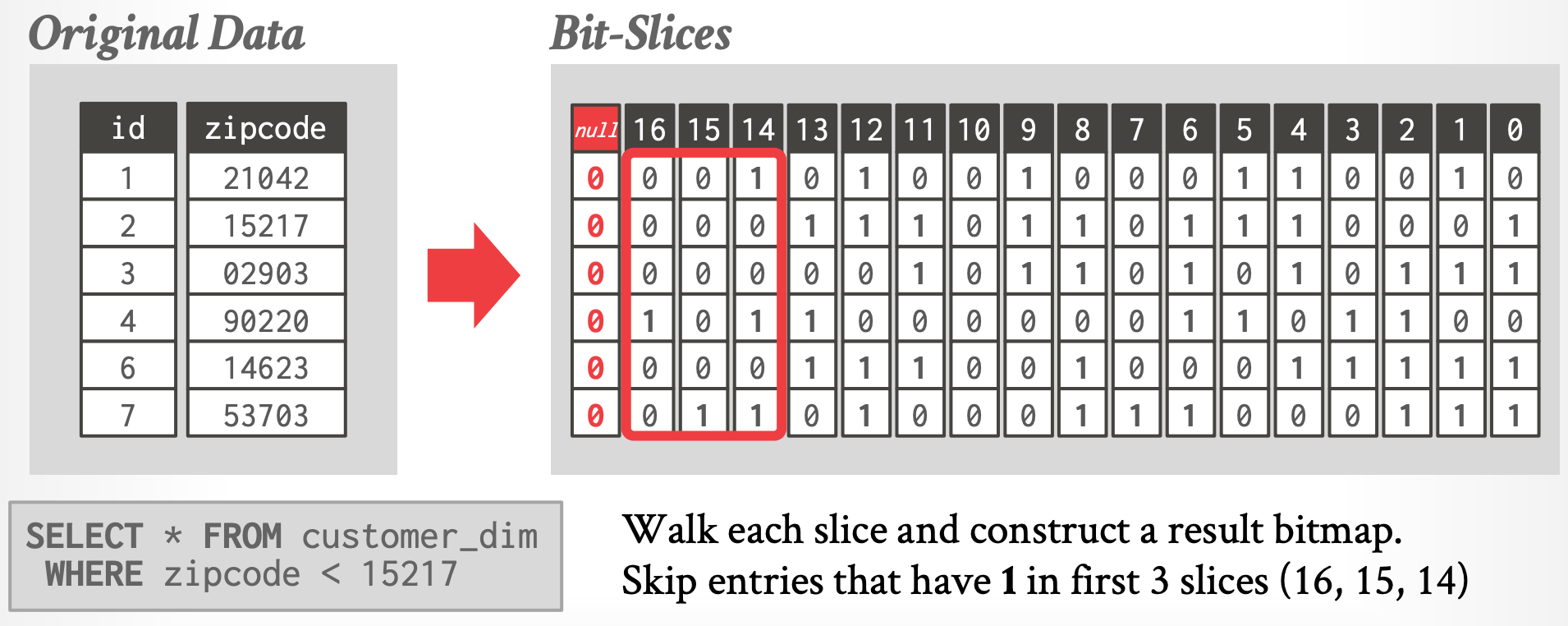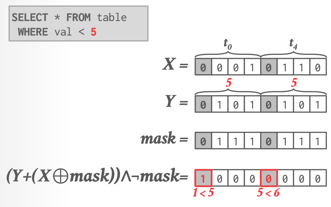其中 $\large bin(21042)→ 001010 0 10001 10 010$ - 将列值对应的 bits 按位拆开，类似行存转列存（一个 bit 可以看作一列），将所有行的第 $i$ 位存储在一起（对应图中，Bitmap/Slice 的方向是**上下**的） - 计算 Predicate 时，一些场景下只比较前面几个 Slice 就能快速 Pruning（如图中例子） - 可以用于高效地进行聚合计算 - 如 `SUM(attr)` 使用 [Hamming Weight](https://en.wikipedia.org/wiki/Hamming_weight) 1. 计算 $slice_{17}$ 中 1 的个数，然后乘以 $2^{17}$ 2. 计算 $slice_{16}$ 中 1 的个数，然后乘以 $2^{16}$ 3. 以此类推... - Intel 在 2008 年添加了 **POPCNT** SIMD 指令，可以计算 1 的个数 - 限制： - 列值的二进制位数不能太多 ## 2.5 BitWeaving - 更现代化的 Bit Sliced - 设计目的：使用 SIMD，在压缩过的数据上可以快速进行 predicate evaluation。 - Bit-level parallelization - 学习材料： - 实现：[Quickstep](https://quickstep.cs.wisc.edu/) - Paper：[BitWeaving: fast scans for main memory data processing](https://dl.acm.org/doi/10.1145/2463676.2465322) - Note: https://dsg.uwaterloo.ca/seminars/notes/2014-15/Patel-Quickstep.pdf - 两种 Storage Layouts： 1. **Horizontal**：Row-oriented storage at the bit-level 2. 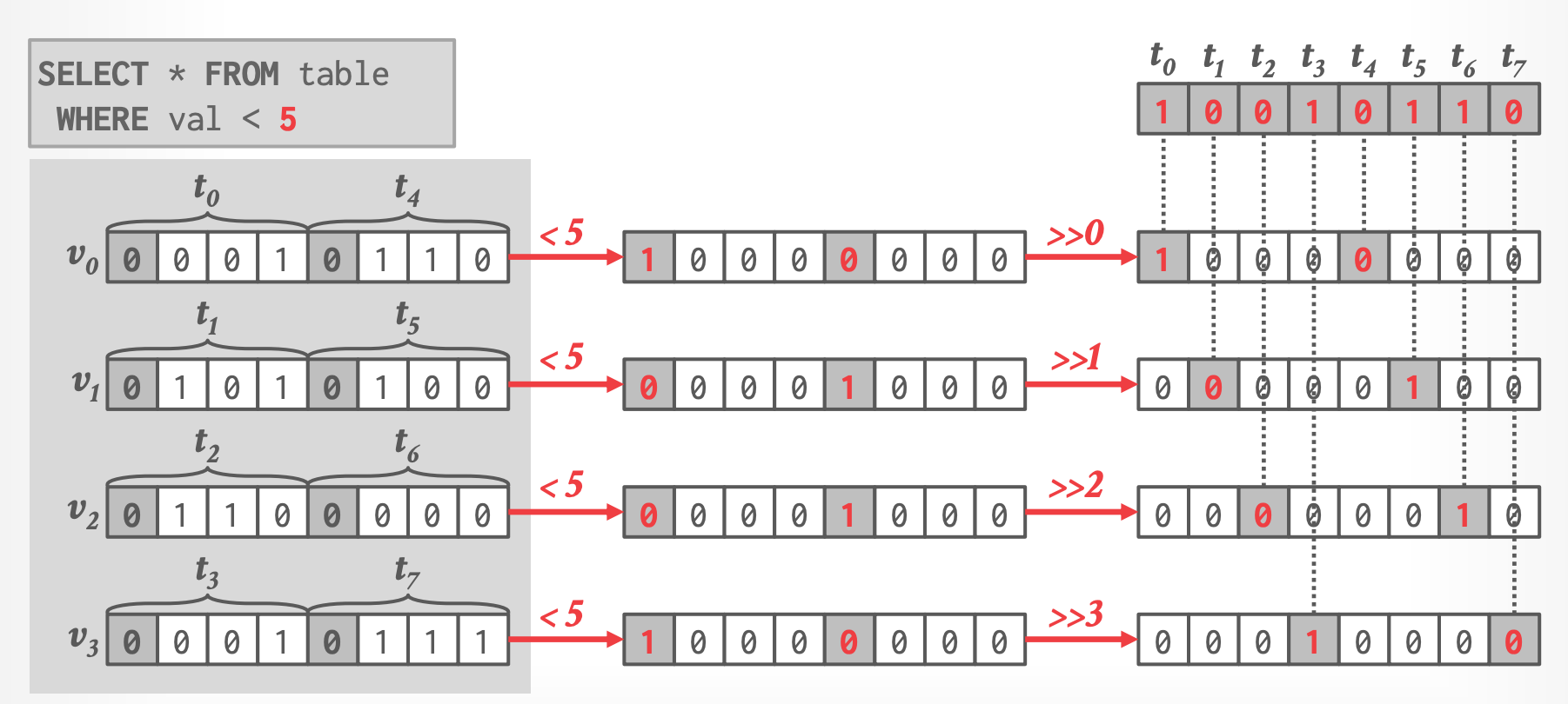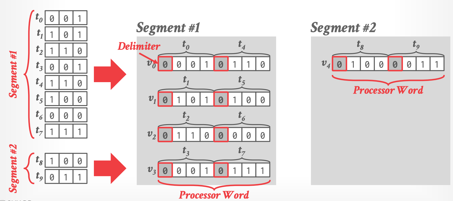**Vertical**：Column-oriented storage at the bit-level ### Horizontal Storage **存储：**  - 图中假设机器字是 8 bits（packed to word） - tuples 是穿插在一起的，如 $t_0$ 和 $t_4$ 在一起。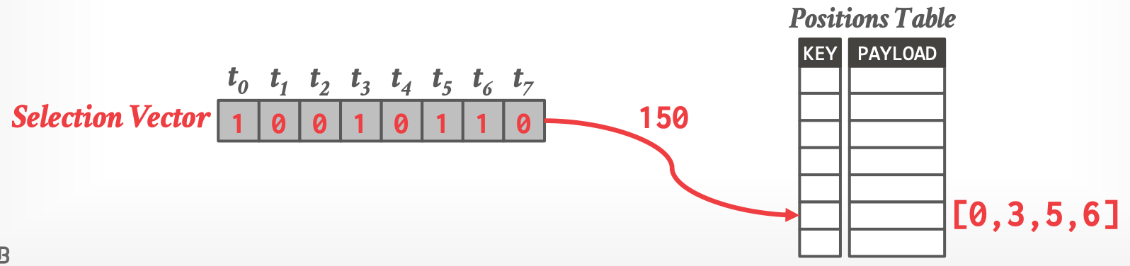 - Delimiter 用于后续的计算 **谓词计算：**  - 计算结果是 selection vector，表示哪些 tuple 匹配到了 - 一个 word 的计算只需要三个指令 - 可以工作于任意的 word size 和 encoding length - 论文里还包含了其他计算的算法  ### Selection Vector - SIMD 比较操作的输出是一个 bit mask，表示了哪些 tuples 满足谓词。 - DBMS 必须将其转化成 column offsets，两种方式： 1. Iteration 2. Pre-computed Positions Table ^e235f5 -  ### Vertical Storage **存储：**  - segment 内所有 tuple 的第 $i$ 位存储打包到一个机器字内 **计算：** 1.  2.  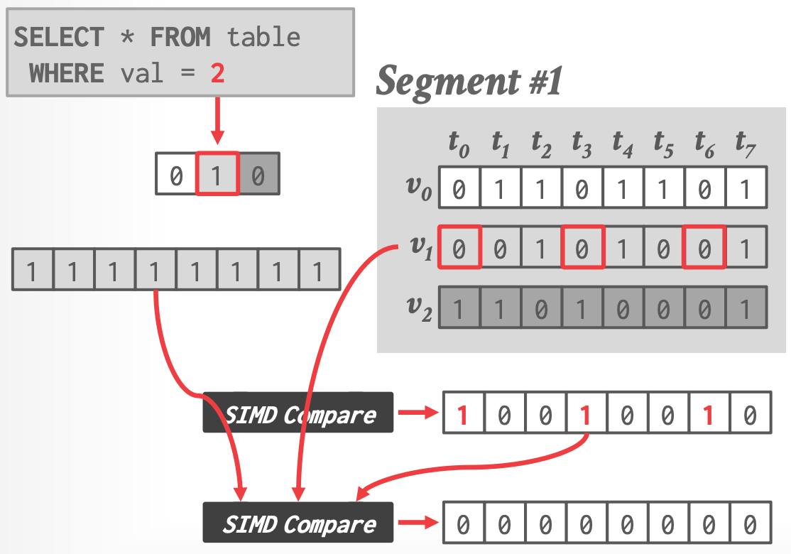- 相比 Horizontal Storage 更高效 - 优势：可以 early quit（如上图中比较结果为 全 0 时） ## Observation - 前面的 Bitmap 机制都是精确/无损的 - DBMS 也可以选择放弃一些精确度，来换取更快的计算速度 - 存在 false positives，还需要查看原始数据 --------- # 3. 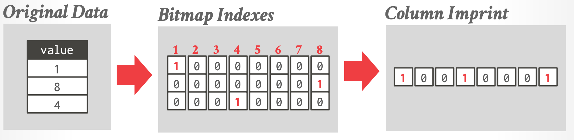Column Imprints  - 从上到下将 bitmap 合并到一起成一个 bitmap - 来判断是否存在某个 value，类似 bloom filter - 论文：[Column imprints: a secondary index structure](https://dl.acm.org/doi/10.1145/2463676.2465306) ---------- # 4. Column Sketches - [[04-olap-indexes#^9b6f0f|range-encoded Bitmap]] 的变种 - Paper：[Column Sketches: A Scan Accelerator for Rapid and Robust Predicate Evaluation](https://dl.acm.org/doi/10.1145/3183713.3196911) - 使用 smaller sketch codes来标识是否存在处于某个范围内的值 - DBMS must automatically figure out the best mapping of codes. - Trade-off between distribution of values and compactness. - Assign **unique codes to frequent values** to avoid false positives.  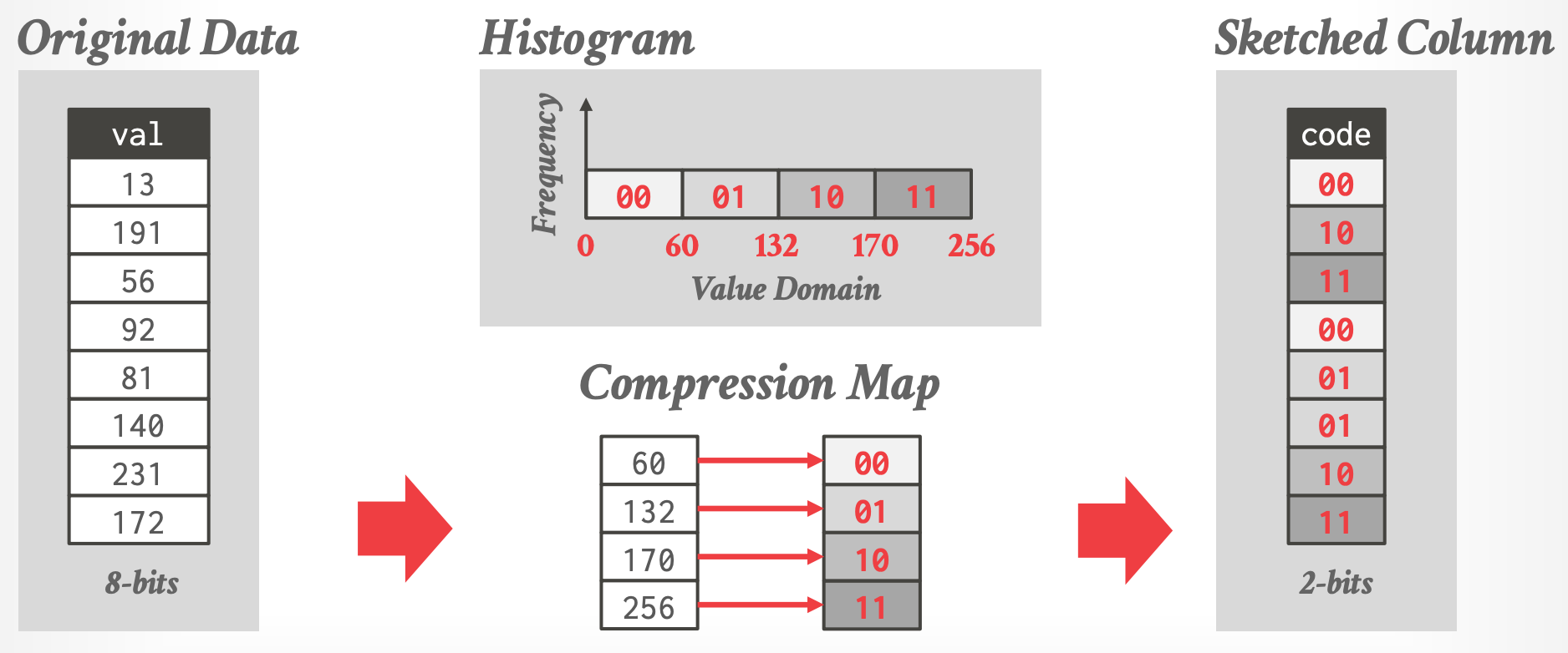- 例如 00 表示小于 60，01 表示 $[60, 132)$ - 不存储原始列值，而是存储 code - 应用：如 `SELECT * FROM table WHERE val < 90`，只需要查找 code 等于 00 和 01 的 ---------- # Parting Thoughts - Zone Maps 被广泛用于加速 sequential scans - Bitmap indexes 在 NSM DBMS 中更常见（相比 columnar OLAP systems）